Principles of loading in Connection, finite element model behind

1 Computational Model

The computational model in Connection, like any other FEM model, has boundary conditions and is loaded in some way. We will describe the structure of the computational model using the concrete example of Connection. Let's consider the following simple plane frame with a connection of a horizontal beam to a column. The beam is loaded with a uniform continuous load, and the moment connection of the beam to the column is rigid, using a front plate. A visualization of the joint is in the following image.

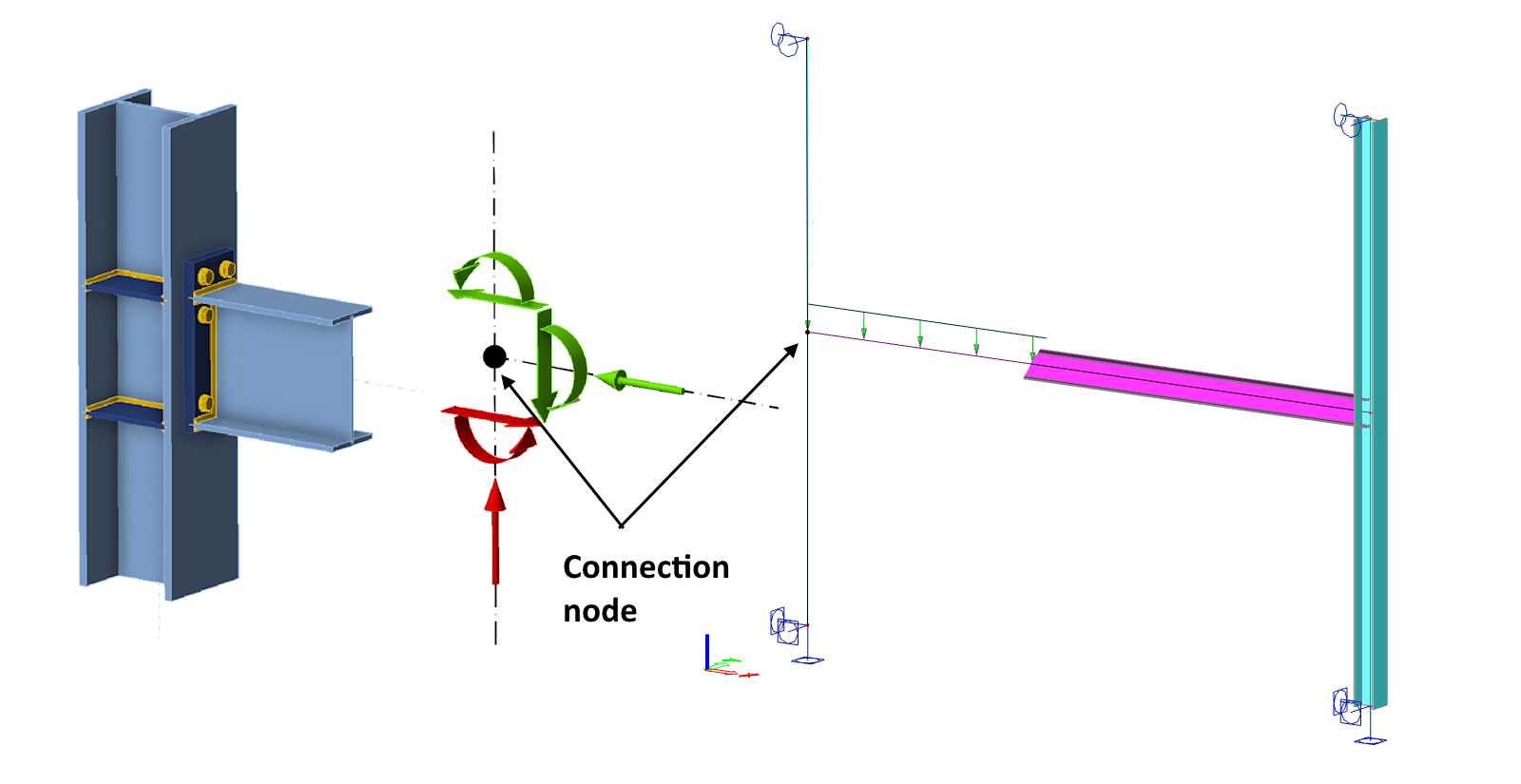
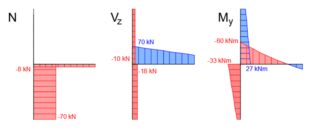
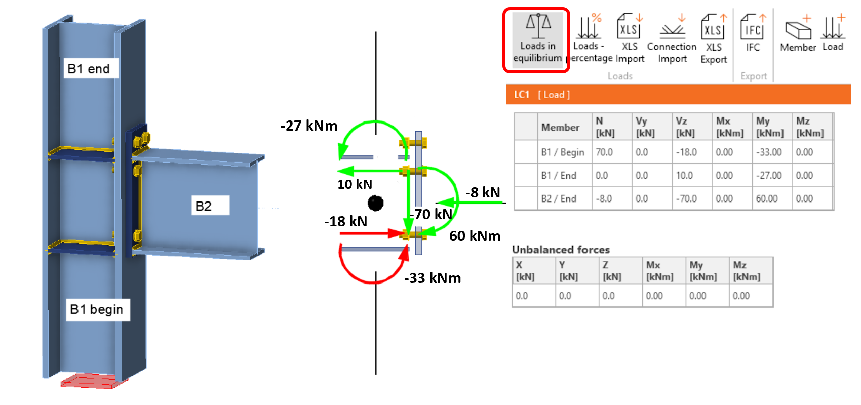
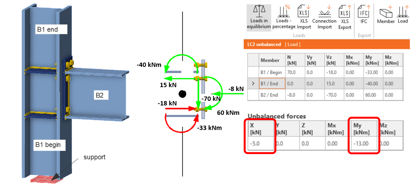
In Connection, the 3D computational model of the contact member is loaded with internal forces acting in the individual members immediately at the connection node (note: in the solid view, the loading forces and moments are displayed at the ends of the visualized connected elements, which can be misleading when using the application for the first time). The center of the connection, represented by a black point in the wireframe view of the connection in the application, is thus identical to the node in the global FEM beam model. The internal forces in members near the analyzed connection, calculated by the global FEA model, are shown in the following figure. The values of the internal forces at the node are given numerically in the figure. 

Two different approaches can be used for modeling of the connection in the application. 

• The connection load is in equilibrium
• The connection load is not in equilibrium

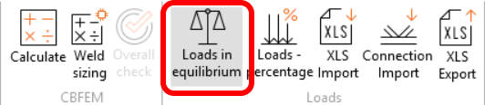
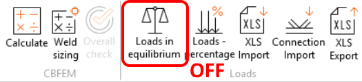
These two approaches differ in the boundary conditions and in the way the computational model is loaded. Two variants of the model are switched using the Loads in Equilibrium button in the Load section of the top ribbon.

Firstly, the article discusses in detail boundary conditions and loading of the analysis model corresponding to the Loads in Equilibrium option.  With this option, the entire connection can be assessed as a whole, and all connected members are loaded. This is the default program setting after a new project is created. 

Boundary conditions and the way of loading the analysis model with the Loads in Equilibrium option turned off will be discussed in detail in section 3. This variant of modeling is suitable, for example, for the checks of the separate connections of individual elements.

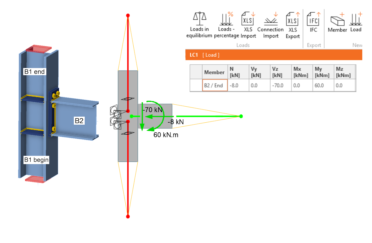
In the Connection application, the model of the studied connection is composed of one continuous member  (column B1) and one ended member (beam B2). The column is set as the bearing member. The computational model is schematically shown in the following image.

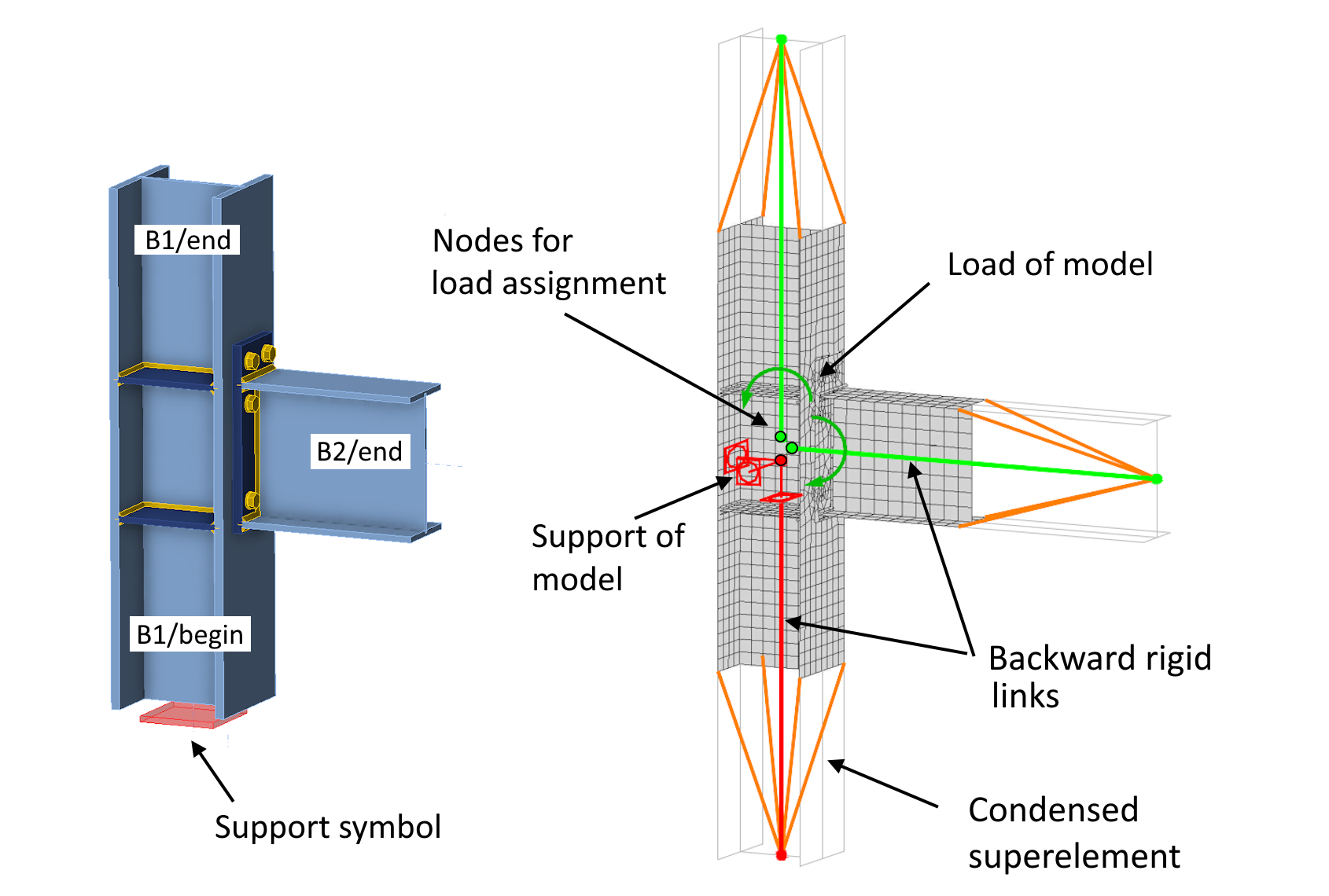
The Finite Element Method (FEM) computational model of the connection consists of:

1. Connected members – a stub of the connected member (beam, column, brace, etc.), adjacent to the joint, is modeled. The cross-section of the element is modeled using shell plastic finite elements.
2. Parts of connection – end plates, gusset plates, stiffeners, ribs, etc. Again modeled using shell plastic elements.
3. CBFEM components – welds, bolts, contacts, MPC (Multi-Point Constraint), etc. These parts of the model are not the main focus of this paper and are described in the theoretical background.
4. Condensed Superelements – ensure the smooth distribution of point loads into the 3D shell model of the connected member. These elements are not visible to users in the scene. They are described in more detail in this article.
5. Backward rigid links – Each end of the connected element (more precisely, the end of the condensed superelement that extends the element) is connected to an auxiliary node at the center of the connection using a backward rigid link. Each rigid link has its own node at the center of the joint. Boundary conditions of the computational model are applied to these nodes, and the connection loading is applied as point forces and moments into these nodes.
6. Supports – boundary conditions of the CBFEM model applied to the starting node of the rigid link.

1.1 Supports

Every FEM computational model needs supports to prevent a singularity. The CBFEM model is fundamentally a general 3D FEM model, which means it requires three supports against translations and three against rotations. As illustrated in the model figure, in our example, a point support (three translations and three rotations) is defined at the starting node of the backward rigid link connecting the lower end of the column and the center of the connection. 

The decision about which member (more precisely, its rigid link) will have the support applied is governed by which connected element is set as the so-called bearing member in the application. The supported end of the bearing element is then visualized using a red square symbol.

1.2 Loading

When using the Load in Equilibrium function, internal forces are set for all members of the connection. A correctly specified load must then satisfy a basic principle: the forces in the connection node must be in equilibrium. Fulfilment of this rule is very important for the correct design of the connection. The application checks that the balance is met and also lists a table of the calculated so-called Unbalanced forces below the table where the load is defined.  If the connection load is defined correctly, the unbalanced forces are zero (or almost zero). The load of our connection is shown in the following figure, the unbalanced forces are zero, so the load is defined correctly. We will discuss the effect of incorrectly specified load when unbalanced forces occur in the model and why they can cause a completely incorrect design of the connection later on with two examples.

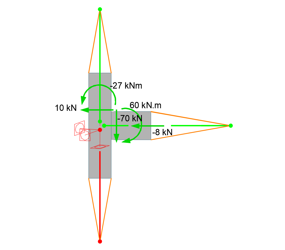
The model loading is applied (like model supports) to the starting nodes of the backward rigid links connecting the connection center and the end of the condensed superelement. In other words, the internal forces in individual members (at the connection center), which were defined in the loading table, are directly set into the computational model. The backward rigid links then ensure that the bending moment from the connection center is transformed to the bending moment at the end of the condensed superelement.

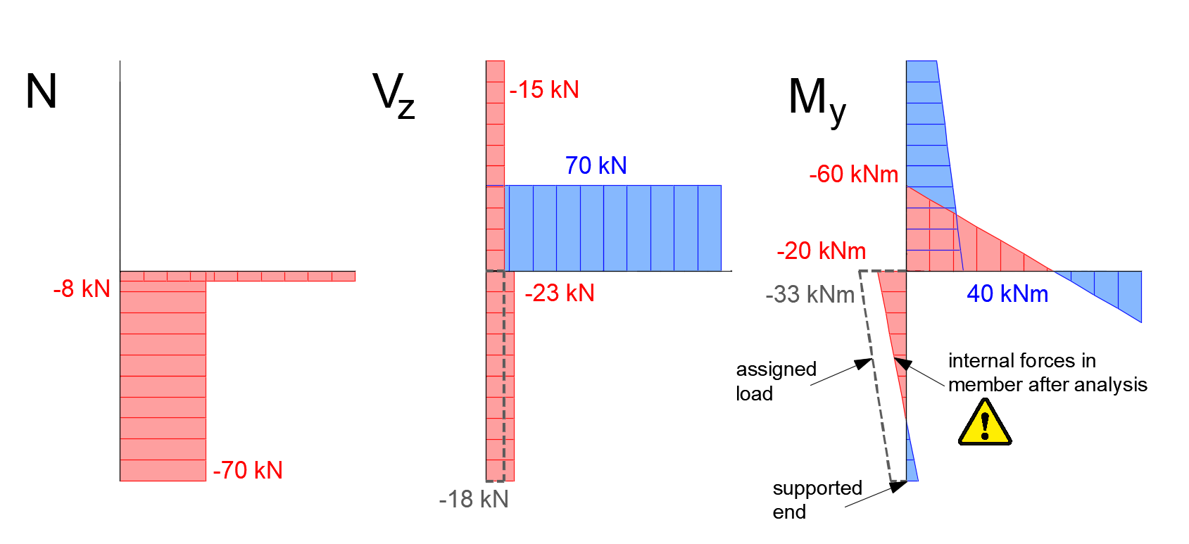
Let's illustrate the function of the backward rigid link more clearly using a simple beam model, where the horizontal member B2 is represented by a simplified beam element instead of the shell 3D model. The internal forces on the member at the center are taken from the example: Vz = -70 kN, My = 60 kN.m. This force and moment are set at the beginning of the rigid link. From there, they are transferred to the end of the condensed superelement and then into the model of the connected element B2. As can be seen, the internal forces in member B2 at its beginning (connection center) are then identical to the inputted point loads.

It is obvious that the resulting 3D computational model is externally statically determinate (only six degrees of freedom are taken) and the model can deform freely without inducing secondary reactions that would change the defined flow of forces. Also, it is clear that specifying loads at the beginning node of the B1/begin backward rigid link, where the model supports are specified, would be useless because the forces and moments would be directly captured by the supports. Thus, the computational model is loaded with forces in B1/end and B2/end, which means only two of the three members are loaded, the third member is supported. However, if the loading of the connection is correct, the specified forces and moments are in equilibrium, the reactions calculated in the B1/begin supports will be identical to the loading defined in the table. The load of the connection computational model is then as follows:

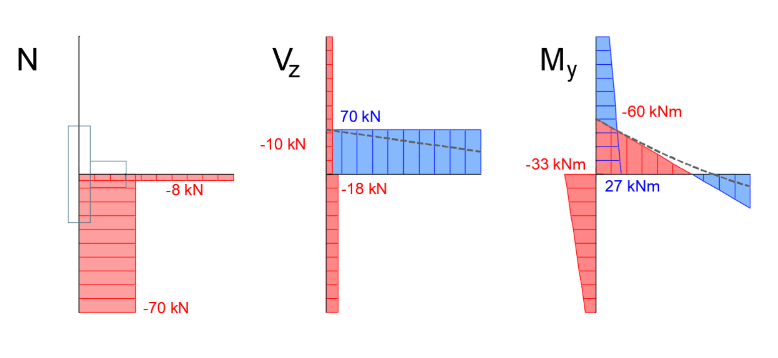
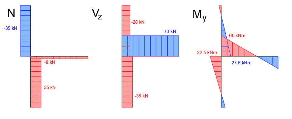
The internal force distribution on the equally loaded and supported beam substitute model is shown in the following figure. Only the forces in the members to be solved are visualized, the backward rigid links are omitted. The internal forces distribution from the global FEM model, which were presented at the beginning of the paper, are also visualized by dashed lines. As can be seen, due to the lack of uniformly distributed loading of the beam in Connection, the moment curve shape is linear compared to the original parabolic one. However, it sufficiently matches the parabolic curve from the global FEM model at the point of connection. Similarly, the shear force in the beam in Connection is constant compared to the linear shape from the global model.

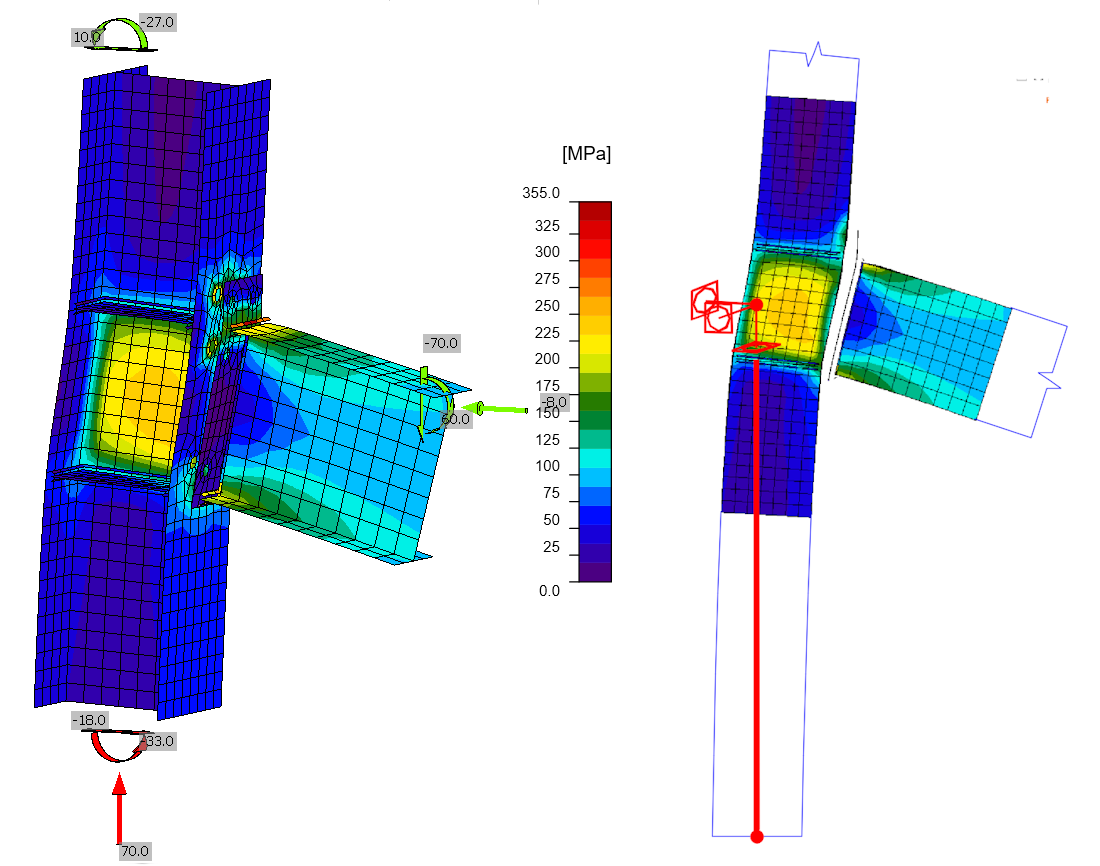
For illustration, the figure below shows the deformed shape after calculation. It is clear from the deformed shape that the model support is at the lower end of the column - through the backward rigid link. In fact, the support in the model is in the middle of the connection.

2 Beware of unbalanced Forces in the connection

We have shown how the FEM computational model of the connection looks in principle, how it is supported, and how it is loaded. In the example above, the specified load was in equilibrium. We will now show the effect on the model loading and connection stress state if the specified load is not in equilibrium. 

2.1 Unbalanced forces in the frame connection

We will use the same example of a rigid frame connection with an endplate. The specified, intentionally incorrect, connection load is shown in the figure below. In the Unbalanced forces table, the program lists the following calculated forces Fx = -5 kN and My = 13kN.m.

The distribution of internal forces in the model under such loading will again be demonstrated using a simplified beam representation of the connection model.

At the bottom of the column (B1/begin, the supported end of the bearing element), the diagram of the bending moment and shear force derived from the forces inputted into the load table are also visualized by a dashed line. It is evident that the bending moments really acting on the column differ significantly from what is specified at B1/begin in the table. These differences correspond precisely to the unbalanced forces of the moment M_y and shear force V_z. Why is that? As already explained, the internal forces specified at the supported side of the bearing member (B1/begin) are not actually applied to the model. Instead, internal forces result from the FEM model calculation as reactions in the supports of the calculation model. And, of course, these reactions are in balance with the load defined at B2 and B1/end. Thus, the effect of unbalanced forces in this example is that the supported bearing element is subjected to entirely different (lower) internal forces than those the user entered into the load table. For this reason, it is necessary to always try to have zero or minimum unbalanced forces in the connection.

For completeness, it should be added that, in this particular case, the horizontal beam connection itself (bolts, end plate, welds) is evaluated correctly because exactly the same load specified for the B2 member in the load table is applied to this member also in the computational model.

2.2 Unbalanced forces in a truss joint

This example illustrates a case where an incorrectly specified load with unbalanced forces in a joint lead to a completely incorrect design of the member connection. We will use the following truss joint, composed of a bottom tension chord, one tension diagonal, and one compression diagonal. The bottom tension chord is interrupted by a bolted assembly joint. For simplicity, we will work only with normal forces in the joint.

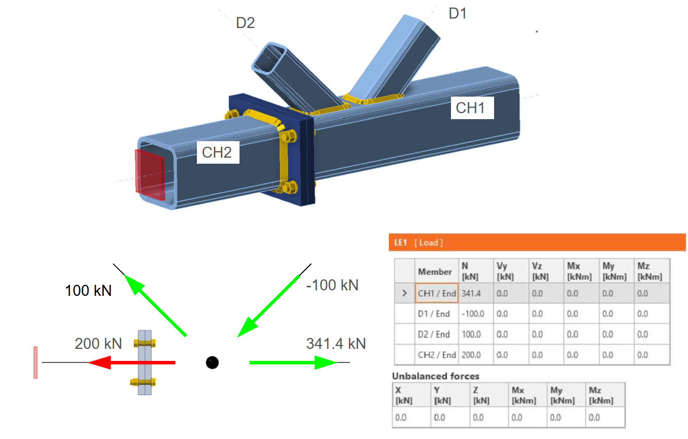
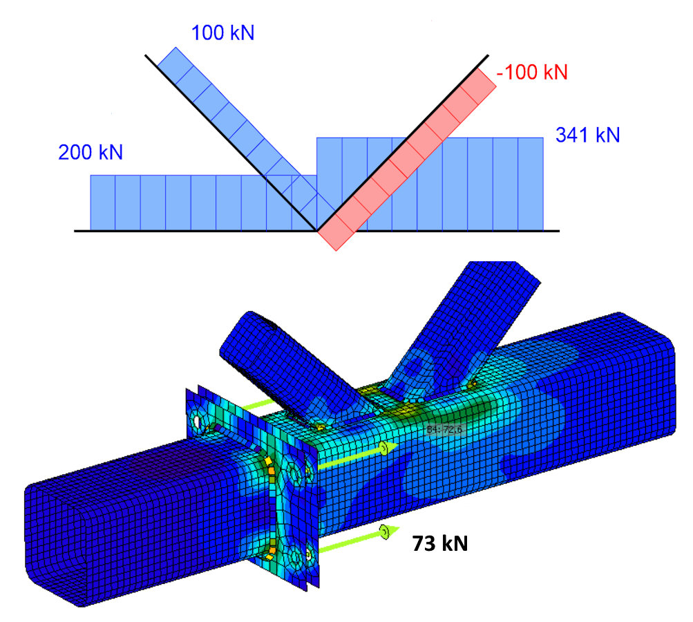
The image above shows a correct specification of balanced internal forces. The resulting normal forces in the truss elements (again using a simplified beam representation of the model) and the tensile forces in the bolts of the assembly joint are as follows. The tensile force in the bolt, including prying effects, is 73 kN.

Now, we will analyze the same joint with unbalanced loading in the horizontal direction X. The loading on the joint is identical to the previous example, except for an incorrectly specified normal force of 240 kN on the bottom tension chord CH1, causing an unbalanced force in the X direction of 101.4 kN.

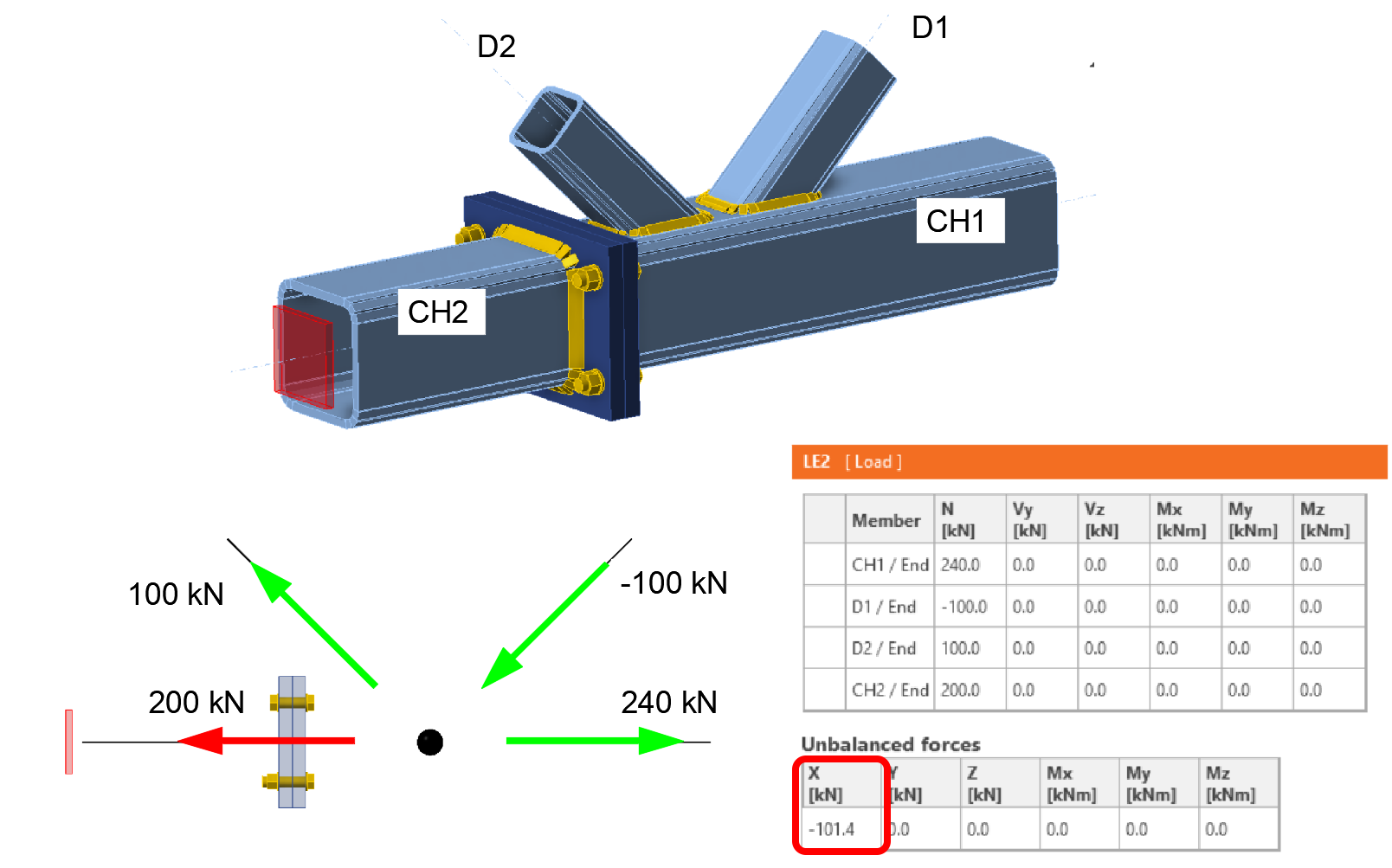
The resulting normal forces in the truss members after the model calculation and the tensile forces in the bolts will be as follows.

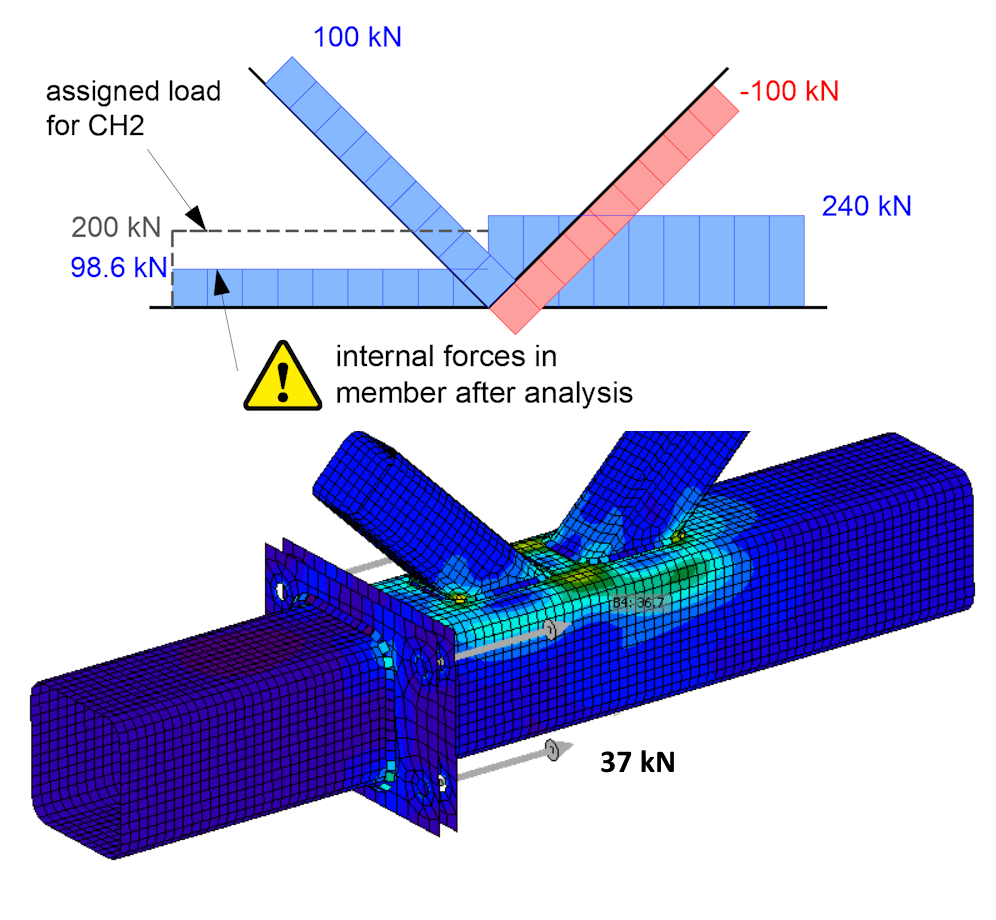
The effect of unbalanced forces in the connection in this example is such that the supported bearing member CH2 is subjected to entirely different (lower) internal forces than those specified in the load table by the user. More importantly, the bolted connection is also checked for a significantly lower tensile force of 98.6 kN than specified in the load table. The tensile force in the single bolt, including prying effects, is 37 kN.

3 Computational model with the Load in equilibrium function disabled

Up to this point, we have been working in the Connection application with the Load in equilibrium function enabled. Now, we will describe the loading and boundary condition of the computational model with the Load in equilibrium function disabled.

We will again use the previously analyzed horizontal beam-to-column connection using a bolted end plate. Disabling the Load in equilibrium function means that the continuous element (column B1) is supported at both ends, and load balance on the beam is not checked. It is also not possible to specify loads in the table for the supported ends of the continuous element (column B1). The only loaded element here is the beam B2. The computational model and the connection's loading looks as follows.

The distribution of internal forces in such a loaded and supported model after the calculation will again be demonstrated using a simplified beam representation of the connection model. The shear force V_z in the beam is divided in the column into a tensile force in the upper part of the column and a compressive force in the lower part. For example, it is clear that achieving a logical distribution of normal forces in the column - where the shear force from the beam would appear as a compressive force directed to the foundations of the frame - is not possible with this model. Similarly, the column's bending moment distribution corresponds to the computational model's support setup and may not reflect the actual internal force flow in the structure.

However, it is important that the internal force distributions in the connected and loaded element B2 are not influenced by the statically indeterminate boundary conditions of the model, and the assessment of the individual element B2 and its connection (end plate, bolts, welds) remains correct. However, the stress state of the column no longer corresponds to the actual behavior in the structure, especially since no loads were applied to it. This shows that disabling the Load in equilibrium function allows the separate assessment of individual members connections. In contrast, with the Load in equilibrium function enabled, the entire connection can be checked, considering the interaction of global effects (e.g., column stress from N+M in the structure) and local effects (e.g., transverse bending of the HEA flange from the bolted end plate connection).