Learning Module: Buckling
Connection design can be difficult to teach, given the detailed nature of the topic and the fundamentally three-dimensional behavior of most connections. However, connections are critically important, and lessons learned in the study of connection design, including load path and identification and evaluation of failure modes, are general and applicable to structural design broadly. IDEA StatiCa uses a rigorous nonlinear analysis model and has an easy-to-use interface with a three-dimensional display of results (e.g., deformed shape, stress, plastic strain) and thus is well suited for the exploration of the behavior of structural steel connections. Building on these strengths, a suite of guided exercises that use IDEA StatiCa as a virtual laboratory to help students learn about concepts in structural steel connection behavior and design was developed. These learning modules were primarily targeted to advanced undergraduate and graduate students but were made suitable for practicing engineers as well. The learning modules were developed by Associate Professor Mark D. Denavit from the University of Tennessee, Knoxville.
Learning Objective
After performing this exercise, the learner should be able to describe how buckling affects the strength of connections and how buckling can be addressed in design using linear buckling analysis.
Background
Successful structural design requires consideration of many physical effects. AISC Specification Section C1 lists 5 major effects that must be considered, including steel yielding, residual stresses, geometric nonlinearity (such as P-δ effects), and initial geometric imperfections.
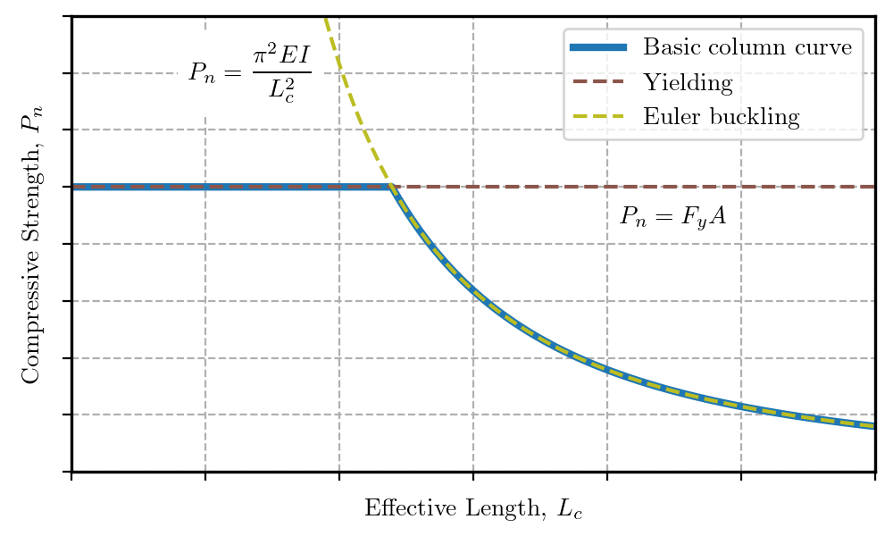
One way these effects are considered in design is with column curves that relate available compressive strength to effective length. A rudimentary column curve for flexural buckling can be established by considering steel yielding and Euler buckling only.
Basic column curve
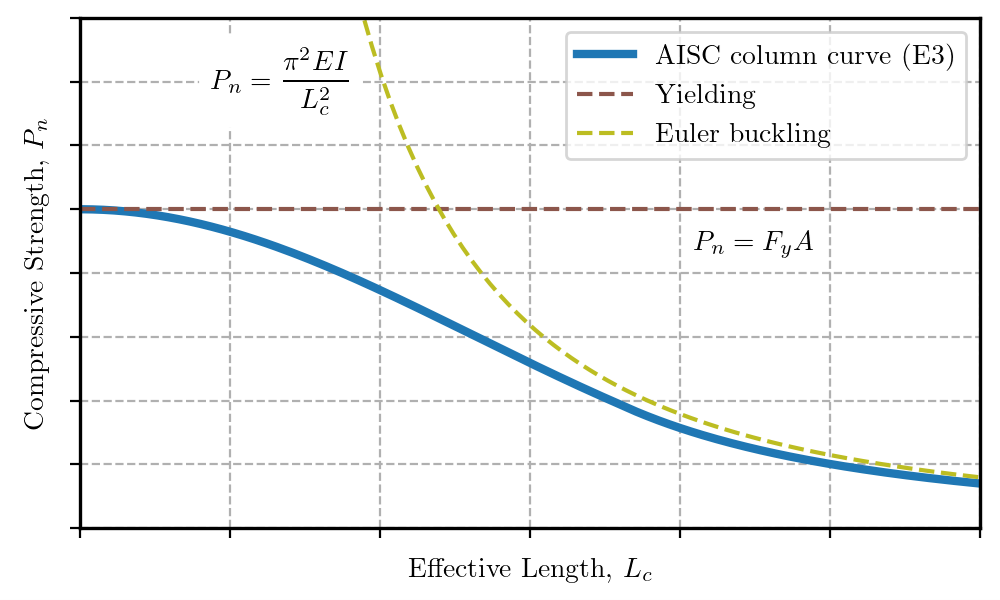
The AISC column curve, defined by AISC Specification Equations E3-2 and E3-3, accounts for residual stresses and initial geometric imperfections, both of which reduce the strength in comparison to the basic column curve.
Column curve defined in AISC Specification Section E3
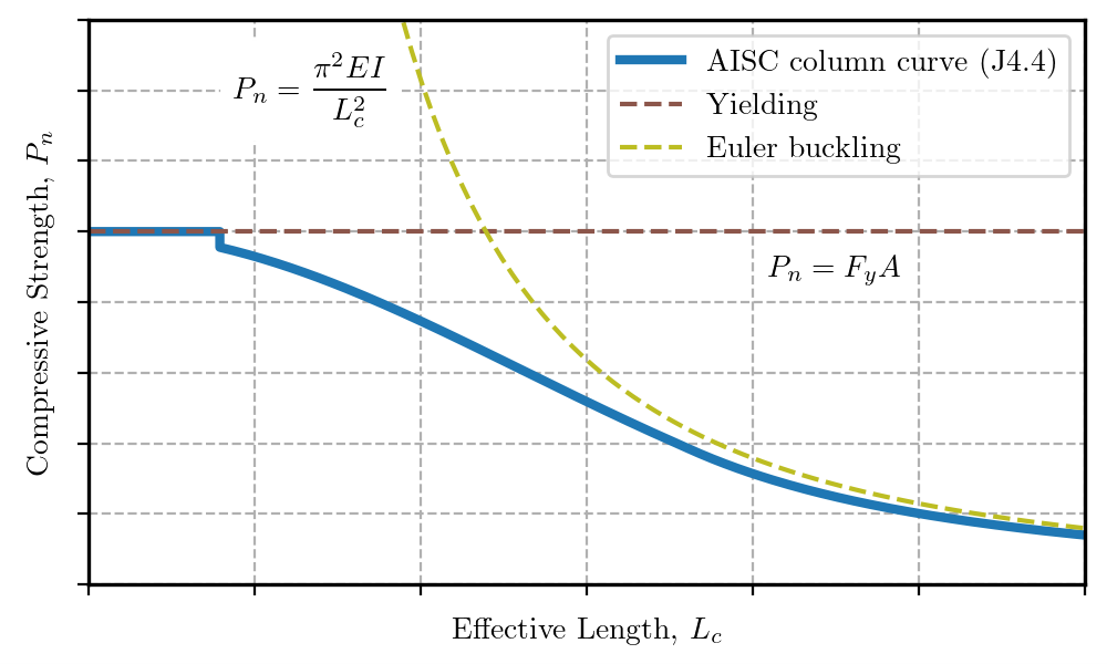
Because connection elements generally have lower residual stresses and different shapes than typical columns, they can achieve higher strengths when the slenderness is low (Dowswell, 2016). AISC Specification Section J4.4 allows the use of a nominal stress equal to the yield stress when the slenderness ratio, Lc/r, is less than or equal to 25.
Column curve defined in AISC Specification Section J4.4
The AISC column curve was developed based on results, for a range of column shapes and lengths, of geometrically and materially nonlinear analysis with imperfections included (GMNIA). This type of nonlinear analysis is considered the truest to reality and can account for all the effects listed in AISC Specification Section C1. A typical IDEA StatiCa analysis is a materially nonlinear analysis excluding the effects of geometric nonlinearity and initial geometric imperfections (MNA). If the connection has a hollow section member as a bearing member, then IDEA StatiCa performs a geometrically and materially nonlinear analysis excluding the effects of initial geometric imperfections (GMNA). For both MNA and GMNA, IDEA StatiCa does not consider residual stresses, which can accentuate stiffness reductions due to partial yielding. Because some physical effects are not considered in the analysis, an additional check for buckling needs to be performed.
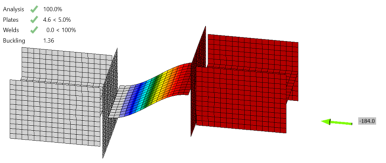
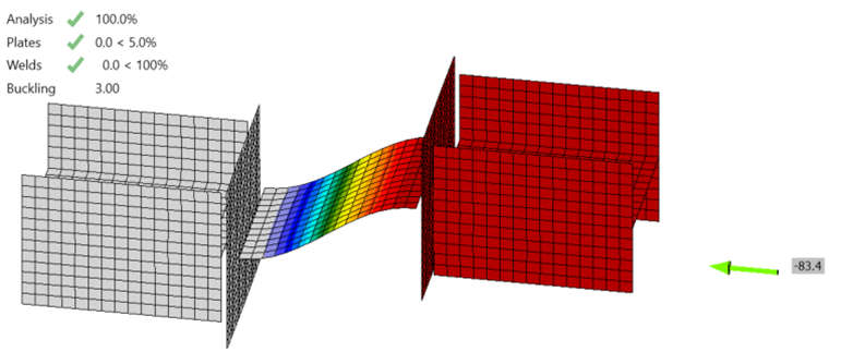
In IDEA StatiCa, buckling is checked using the ratio between the critical buckling load and the applied load, termed the buckling ratio or buckling factor, αcr. The buckling ratio must be greater than or equal to a minimum, limiting buckling ratio. The limiting buckling ratio, αcr,lim, depends on the type of buckling (e.g., global buckling vs local buckling) and material properties. It also depends on the design method used (i.e., LRFD vs ASD). A general recommendation for local buckling is that the buckling ratio should not be less than 3.0 for LRFD or 4.5 for ASD.
Buckling can be more accurately assessed in IDEA StatiCa by reducing the yield strength by a factor that depends on slenderness as described in this article. However, this approach is not commonly used in practice.
Connection
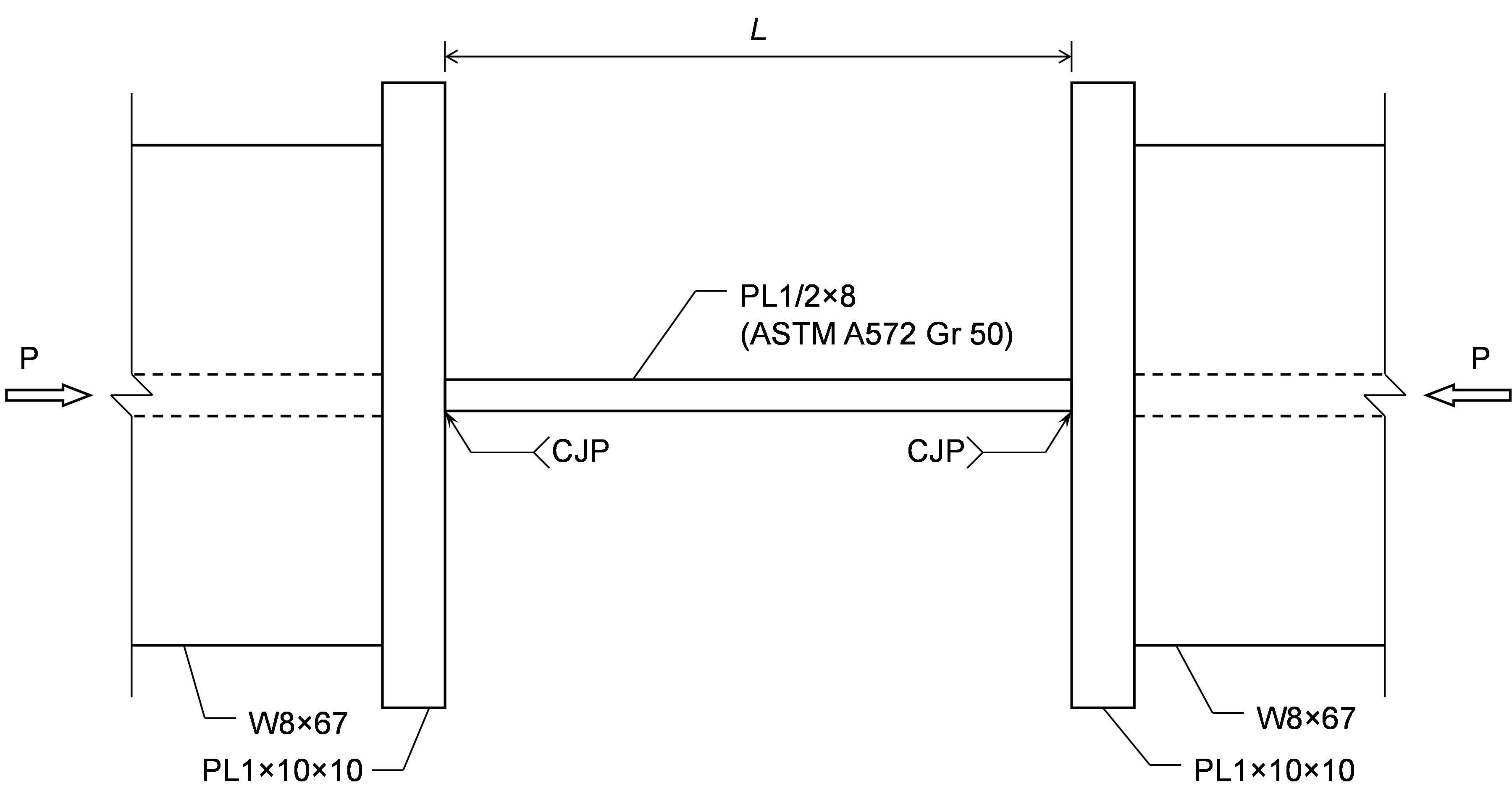
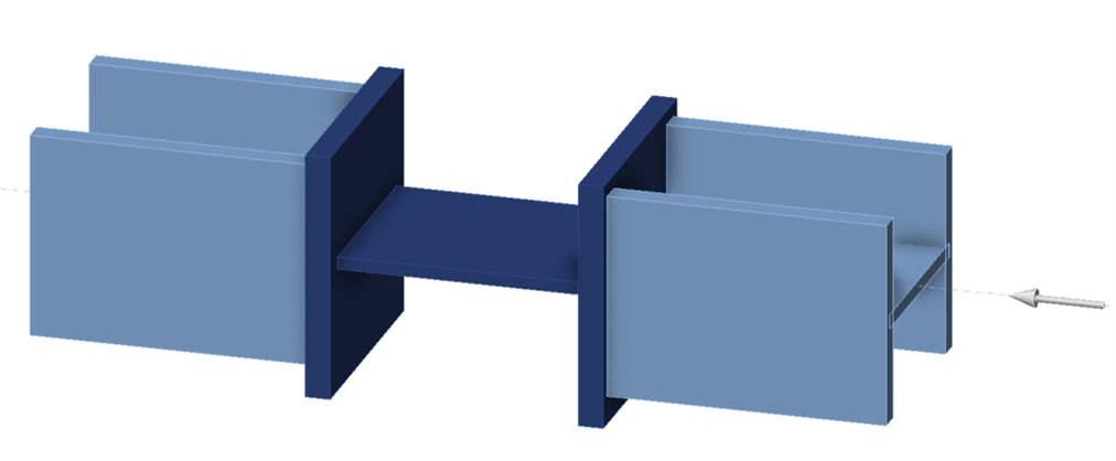
The connection examined in this exercise consists of a 1/2 in. thick by 8 in. wide plate between two W8×67 members, each with a thick end plate. While not a practical connection, the configuration enables comparison of analysis results to hand calculations.
The length of the connection plate, L, can be adjusted in the model provided with this exercise using the position of the end plates (operations SP1 and SP2).
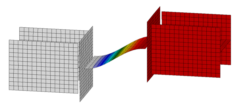
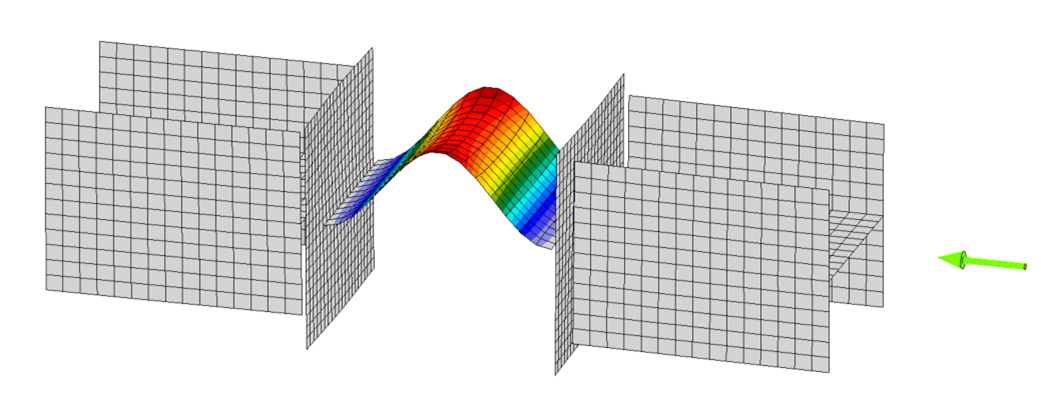
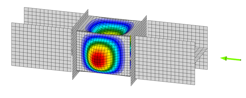
Member B2 is set as the bearing member. Member B1 is assigned a “N-Vy-Vz” model type to prevent rotation of the W8 in both stress/strain (EPS) and buckling analyses. The resulting buckled shape is shown below. With these boundary conditions, the effective length factor, K, equals 1 and the effective length of the plate, Lc, equals the unsupported length, L.
Procedure
The procedure for this exercise assumes that the learner has a working knowledge of how to use IDEA StatiCa (e.g., how to navigate the software, define and edit operations, perform analyses, and look up results). Guidance for how to develop such knowledge is available on the IDEA StatiCa website.
Retrieve the IDEA StatiCa file for the example connection provided with this exercise. Open the file in IDEA StatiCa. To perform the exercise, follow the narrative, complete the tasks, and answer the questions.
Examine the connection with length, L = 10 in.
Examine the connection with various lengths.
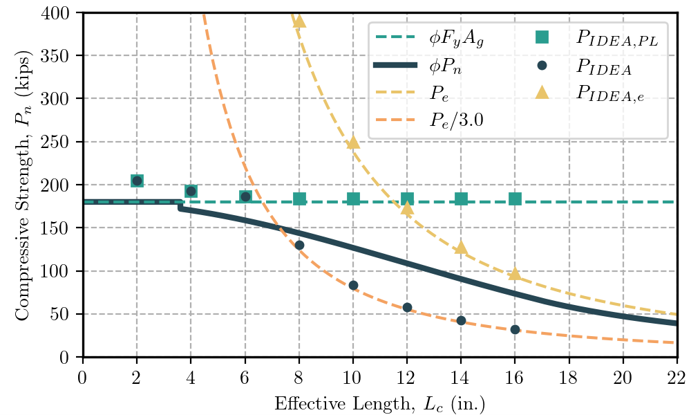
Complete the table shown below, where Pe is the Euler buckling load, ϕPn is the design compressive strength according to AISC Specification Section J4.4, PIDEA,PL is the maximum permitted applied load from IDEA StatiCa considering only the 5% plastic strain limit, PIDEA is the maximum permitted applied load from IDEA StatiCa considering the 5% plastic strain limit and a limiting buckling ratio of 3.0, and PIDEA,e is the buckling load from IDEA StatiCa. Plot the results versus effective length, Lc.
| L = Lc | Lc/r | ϕFyAg | Pe | Pe/3.0 | ϕPn | PIDEA,PL | PIDEA,e | PIDEA |
| in. | --- | kips | kips | kips | kips | kips | kips | kips |
| 2 | 13.9 | 180.0 | ||||||
| 4 | 27.7 | 180.0 | 1,490.7 | 496.9 | 170.2 | 193.0 | 1,522.8 | 193.0 |
| 6 | 41.6 | 180.0 | ||||||
| 8 | 55.4 | 180.0 | 372.7 | 124.2 | 143.8 | 184.0 | 390.0 | 130.0 |
| 10 | 69.3 | 180.0 | ||||||
| 12 | 83.1 | 180.0 | 165.6 | 55.2 | 108.6 | 184.0 | 173.7 | 57.9 |
| 14 | 97.0 | 180.0 | ||||||
| 16 | 110.9 | 180.0 | 93.2 | 31.1 | 73.3 | 184.0 | 97.2 | 32.4 |
Other Connections
You can further explore the effects of buckling and the characteristics of design for stability using linear buckling analysis by analyzing other connections. The following other connections are suggested for further exploration.
Connection 2
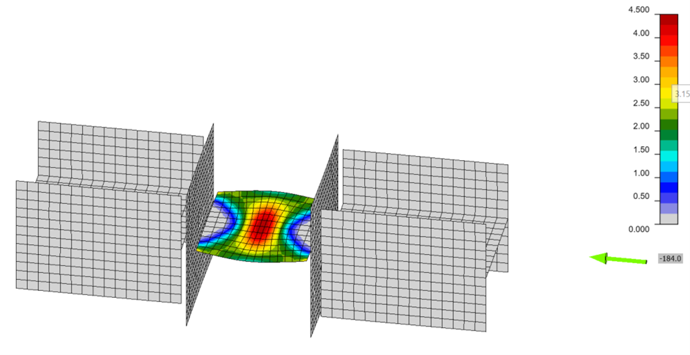
The connection used in the procedure above, but with lateral restraint such that the plate buckles in a fixed-fixed (K = 0.5) mode. This restraint is achieved by setting the model type for both members to “N-Vy-Vz-Mx-My-Mz”.
Connection 3
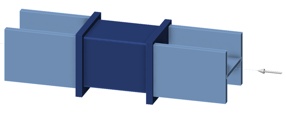
The connection used in the procedure above, but with the plate replaced by a thin square hollow structural section to evaluate local buckling. Adjust slenderness by changing the thickness of the hollow structural section. Reference AISC Specification Section E7 for provisions on local buckling of hollow structural section compression members.
Connection 4
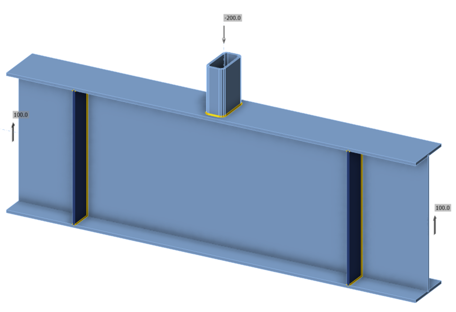
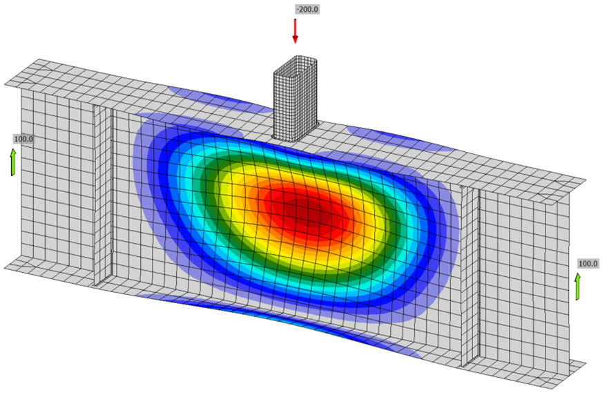
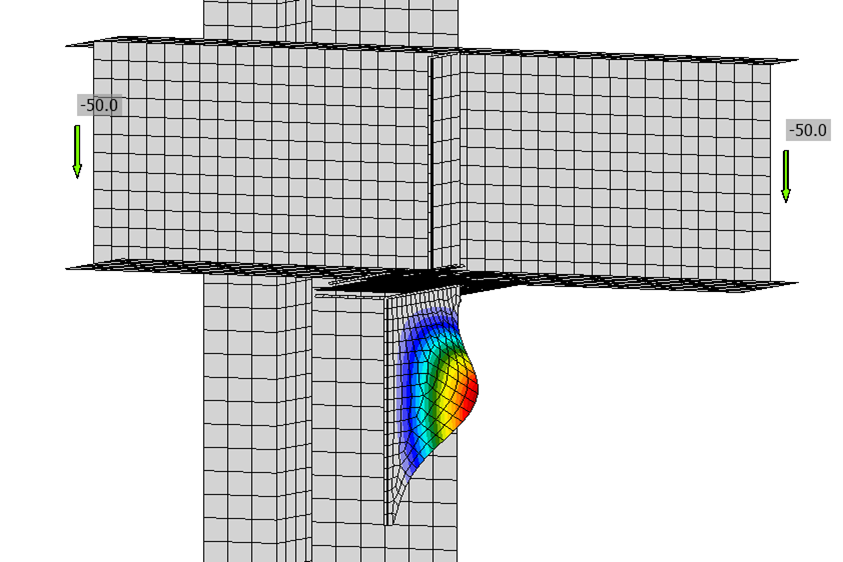
A wide flange beam with a point load to evaluate web local crippling. Adjust slenderness by changing the thickness of the web of the wide flange. Reference AISC Specification Section J10 for provisions on flanges and webs with concentrated forces.
Connection 5
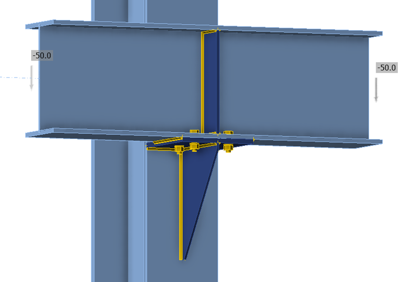
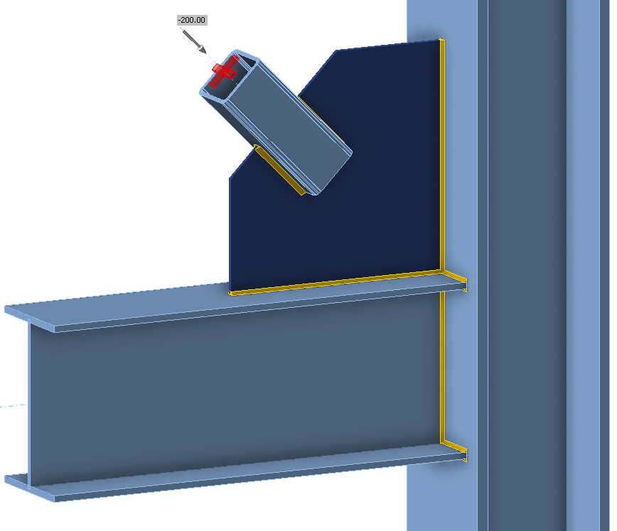
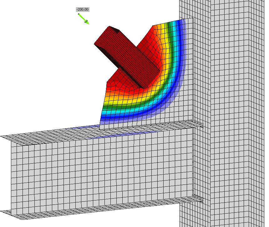
Connection with a triangular bracket plate. Adjust slenderness by changing the thickness of the bracket plate. Reference AISC Manual Part 15 for guidance on the design of bracket plates. Additional guidance can be found in Dowswell and Vild (2023) and this article.
Connection 6
Gusset plate connection in a braced frame. Adjust slenderness by changing how far the diagonal brace is away from the work point. Reference AISC Design Guide 29 Appendix C for guidance on buckling of gusset plates.
References
AISC. (2022). Seismic Provisions for Structural Steel Buildings. American Institute of Steel Construction, Chicago, Illinois.
AISC. (2023). Steel Construction Manual, 16th Edition. American Institute of Steel Construction, Chicago, Illinois.
Dowswell, B. (2016). “Stability of Rectangular Connection Elements.” Engineering Journal, AISC, 53(4), 171–202. https://doi.org/10.62913/engj.v53i4.1106
Dowswell, B. and Vild, M. (2023). “Linear buckling analysis in the design of bracket plates.” ce/papers, 6(3–4), 1831–1836. https://doi.org/10.1002/cepa.2631
Muir, L. S. and Thornton, W. A. (2014). Vertical Bracing Connections – Analysis and Design. Design Guide 29, American Institute of Steel Construction, Chicago, Illinois.


